Taxes and the IS-LM Curve: A Relationship

By Saifullah Penick and Thomas Piwonka 

Quite often, arguments over increased government spending as opposed to tax-cuts are made common, a false polemical implication of an opposition as both are expansionary policies. For example, the Trump administration enacted tax cuts in 2017 which in 10 years will benefit each fifth of the U.S. economy, ordered from richest to poorest, with the following percentage income increases as a result of the tax-cut (Coy, 2020) :

2.3 %  - Richest fifth

1.4 %

1.3 %

0.9 %

0.3 %  - Poorest fifth

GDP in 2018 rose by about 0.8 percentage points and job growth by 0.24 per percentage points as a result (Coy, 2020). In pursuit of a better understanding regarding tax policy, let us examine the IS-LM model which is composed of an IS curve and an LM curve.

Directing now to the Investment-Savings (IS) curve, we see that the increase in GDP is well incorporated and predicted as a result of a tax cut. The assumption is made that demand is equal to output and that output is equal to consumption (as a function of income after tax), government spending, and investment (as a function of output and investment). From this, a tax cut increases disposable income and thereby consumption. Increased consumption is an increase in demand which will be met by an increase in supply. Increase in demand, or sales, will increase investment because the increase in investment will help suppliers rise to meet the new demand; however, depending if interest rates are high such that the investment will not make positive returns for the investor, then the investment will not be made. In sum, tax-cuts stimulate demand which suppliers then try to meet, increasing GDP. The following graph demonstrates the inverse, such that if taxes are raised then the level of output at any given level of interest decreases.

Illustration1:

LM CURVE

The LM curve, or Liquidity Preference-Money Supply curve,  is represented on the graph by the horizontal axis labeled LM. 

Illustration2:

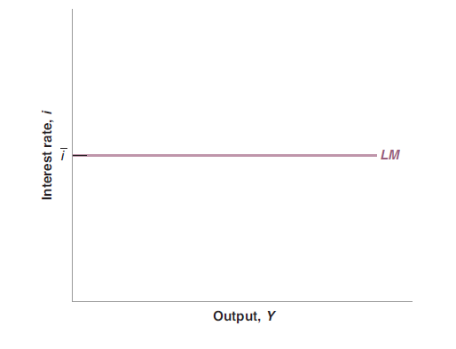
Essentially what this is is the monetary policies which are the result of choosing an interest rate (Blanchard 2016 pg 115) . In effect the government will buy or sell securities as a way of increasing or decreasing the interest rate at any given time.  An example of this would be the debt auction in hungary which took place in 2016, when 233 million  worth of debt was sold, which in turn increased the interest rates from 3.12 to 3.29.(Margit Feher, Wall Street Journal 2016)  This on our graph would be shown as an upward shift in the LM curve.  This use of monetary policy when combined with the IS curve gives us a detailed account of how the goods market interacts with the money market.

IS-LM

The IS-LM curve is a Keynesian macroeconomic model that shows how the market for economic goods (IS) interacts with the Loanable funds market (LM) or money market.  (investopedia 2020) Basically what is shown in the graph below depicts the relationship between these two economic variables, which by varying degrees are controlled by different monetary and fiscal policies.

Illustration3:

The relationship basically entails that a shift of the LM curve down would cause the equilibrium output and interest rates to expand and contract accordingly. For example when a government decides to decrease the interest rate they will buy securities and as a result more money will be placed back into the economy, and liquidity will also increase.  This is shown on the graph below, and as you will notice the new equilibrium output and Interest rate will be lower and the output to be higher, signaling an economic growth (Blanchard 2016 pg 118).

Illustration4:

Harking back to tax policy, we know how tax affects the IS curve, but is there a case to be made where it may affect the LM curve? Yes, if broader definitions of the money supply like M3 money supply are used. M3 money supply is the broadest definition of money supply and includes “near money,” or assets which are less liquid than cash , viewing money as more of a store of value and not so much a medium of exchange; though, let it be noted that most institutions have not used this definition since 2006 because of better modeling using only the most liquid definition of money (cash, checking and savings, and money market funds) as well as problems caused by giving less liquid factors of M3 equal weight to more liquid factors (Chen, 2020). It then follows if tax policy can skew financial markets so that illiquid or liquid assets are favored then transfers from illiquid assets to liquid assets increase the money supply and the other way decrease the money supply. Tangentially, so long as value is wrapped up in assets, the velocity of money is slowed thereby suppressing demand thereby suppressing output. Returning to the point, “because of the asymmetric taxation of liquid and illiquid assets [...]  low-rate taxpayers collect rents from holding high-return illiquid securities [...] regardless of their cash needs,” (Listokin 2011). Here Listokin points out existing tax incentives for the holding of illiquid assets, the market for high-return illiquid assets is artificially increased and (by our assumptions) restricts the money supply. Under a different scrutiny, for, “the federal income tax [...] the investor’s preferences change...after taxes, holding real estate no longer enables the investor to purchase the same amount...as cash does. As a result the investor prefers to hold cash,” (Listokin 2011). This points out a contrasting force in fiscal policy from Listokin’s first point which favors liquid markets and (by our assumptions) increases the money supply, resulting in a model which would explore equilibria between these two forces and how fiscal policy might give economists another tool with which to manipulate markets when needed. It also implies one fiscal policy implementation will affect the IS curve, as discussed earlier, and the LM curve, through money supply as discussed in here ending in a new equilibrium for interest rates.

Understanding this connection between fiscal policy and the LM-IS curve allows us to think of alternative ways of affecting the market in a scenario where it has crashed, however it should be noted that these policies do not always work, and it invites the question of how much these policies can actually accomplish.

Citations:

Coy, Peter. Bloomberg.com, Bloomberg, 27 Oct. 2020, 8:42, www.bloomberg.com/news/articles/2020-10-27/the-trump-tax-cut-wasn-t-just-for-the-rich.

 

Feher, M., & Bartha, E. (2016, Oct 13). Hungary bond auction receives solid demand; robust demand follows an upgrade of hungary's debt and increased liquidity from a planned easing of monetary policy. Wall Street Journal (Online) Retrieved from https://ezproxy.plu.edu/login?url=https://www-proquest-com.ezproxy.plu.edu/newspapers/hungary-bond-auction-receives-solid-demand-robust/docview/1828168874/se-2?accountid=2130

 LISTOKIN, YAIR. “Taxation and Liquidity.” The Yale Law Journal, vol. 120, no. 7, 2011, pp. 1682–1732. JSTOR, www.jstor.org/stable/41149577. Accessed 11 Mar. 2021.

Staff, Investopedia. “IS-LM Model.” Investopedia, Investopedia, 26 Oct. 2020, www.investopedia.com/terms/i/islmmodel.asp#:~:text=The%20IS%2DLM%20model%2C%20which,(LM)%20or%20money%20market.