How Does Government Stimulus Affect Unemployment?

    Sadie Brownlee and Charlie Cutter

A prevalent topic in the news during the pandemic has been skyrocketing unemployment across the world and numerous governmental tactics to combat it. The threats of high unemployment on the employed and the searching are twofold: fewer jobs available mean people are less likely to find a job, and that employed people are at more risk of losing their jobs (Blanchard). Thus, governments should keep their unemployment rate low and maintain employment to avoid great economic shocks that have the potential to spiral. For reference, the Great Recession saw a peak close to 10% unemployment, with the percent unemployed finding a job dropping from 28% to around 17%. 

Fig. 1 - The Unemployment Rate and the Proportion of Unemployed Finding Jobs, 1996-2014

Source: Blanchard 142

Fig. 2 - The Unemployment Rate and the Monthly Separation Rate from Unemployment, 1996-2014

Source: Blanchard 143

Government stimulus directed towards the unemployed reduces the decline in real wages. Higher unemployment leads to lower real wages as workers have a weaker bargaining position (Blanchard). Unemployment insurance makes unemployment less painful and reduces the drop in real wages by allowing the worker some or more of their prior wage, in the case of added stimulus. By providing some of the worker’s previous wages, the drop in consumer demand is dampened, decreasing unemployment’s adverse effects on the economy. The Great Depression was the catalyst for the establishment of unemployment insurance in the US, where estimates place unemployment higher than 20 percent (Pells).

Fig. 3 - Unemployment Rate, Seasonally Adjusted        

Source: Australian Bureau of Statistics

Fig 4. - Changes in payroll jobs, mid‑March to end‑May 2020  (indexed)

Source: Australian Government

Similar to graphs we have seen from the United States, the Unemployment Rate of Australia skyrocketed during the pandemic with a peak of 7.5% in July of 2020. The pre-pandemic rate in February of 2020 was 5.1%. JobKeeper is a wage subsidy program implemented by the Australian government designed to give businesses the ability to maintain their employees’ wages without laying off many, if any (Australian Government). It is one of many ways governments are attempting to curb rising unemployment. As Fig. 4 demonstrates, unemployment plateaued after the introduction of JobKeeper.  After a year and over $68 billion spent, the Australian government is terminating the program, inciting alarm from some and relief from others (Heath). Some Aussies believe the program has been successful and does not need to continue (Heath). Throughout 2020, 875,000 new jobs were created, with only one month where jobs were lost (Heath). This month of contraction, September, coincided with the Australian state of Victoria’s second wave of COVID-19 (Heath). Economists suggest this overall growth will absorb any loss the country will incur upon the end of the subsidy (Heath). However, not everyone is so convinced. According to Diana Mousina, senior economist at AMP Capital Investors Ltd, 1.3% of the workforce is underemployed, indicating that the economy has much more room for growth under the protection of JobKeeper (Heath). Without it, this portion of the workforce is at a high risk of unemployment (Heath). Some economists land in the middle, stating that broad wage subsidies should end, but more targeted stimulus should continue (Duke). But will targeted stimulus provide as much relief as people hope?

A study conducted by Ursula Jaenichen and Gesine Stephan suggested targeted wage subsidies for “hard-to-place” workers, such as those who have been unemployed for extended amounts of time or disabled people, can stimulate employment but can also be associated with some deadweight loss (Jaenichen). They found the share of “hard-to-place” workers that took on a subsidized job, as opposed to remaining unemployed, was 25-42% greater than their unsubsidized counterparts (Jaenichen). In other words, 25-42% of those employed in a new job after being introduced to the workforce through subsidized employment would not have been employed without this opportunity (Jaenichen). However, compared to those that went straight into unsubsidized employment, rather than beginning with a subsidized job and transitioning out, the latter was not better off than the former and incurred a deadweight loss (Jaenichen). Therefore, their study found that being employed through a subsidized program is much better than being unemployed but not any better than having an unsubsidized job (Jaenichen). For Australia, this study supports maintaining wage subsidies, i.e., the JobKeeper program, for people who would not otherwise be able to find employment. For those that can easily find a job, wage subsidies are unproductive.  

Additionally, the effects of targeted labor stimulus are challenging to isolate and quantify due to numerous measurement factors, such as defining labor markets and whether they should overlap. Manning and Petrongolo conclude that an increase in job vacancies in one area, as well as a decrease in the cost of the distance between a job and home (calculated separately and independently in their study), both radiate far beyond the targeted locale for these programs (Manning). They found that localized efforts to meet labor demand prompt people in other areas to redirect their job searches, therefore expanding the affected region, as fig. 5 illustrates for the London suburb Stratford (Manning). Manning and Petrongolo highlight that not allowing for overlapping labor markets or improperly measuring the affected zone’s size can skew results toward overestimating or underestimating the stimulus’s impact (Manning). This means that focusing aid to specific parts of Australia that need more support than others may not be as potent as necessary to prompt a strong recovery, or the data reported may not accurately reflect its impact. 

Fig. 5 - The Effect of a Doubling in the Number of Vacancies in Stratford, England, on the Unemployment Outflow (Percentage change)

Source: Manning

Fig. 6 - The Effect of Halving the Cost of Distance Between Heathrow and Stratford on the Unemployment Outflow (Percentage Change)

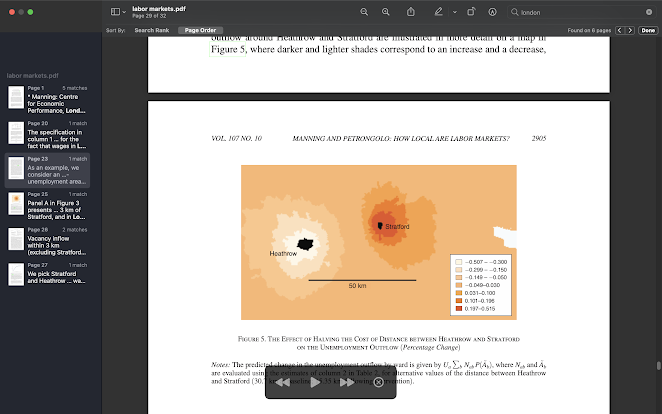
Source: Manning

Context: Stratford is a high-unemployment area in East London, while Heathrow is a low-unemployment area 30.7 km away or 1 hour and 20 minutes drive.

Works Cited

Blanchard, Olivier. Macroeconomics. 7th ed., Pearson Education Inc., 2017. 

Manning, Alan, and Barbara Petrongolo. “How Local Are Labor Markets? Evidence from a Spatial Job Search Model.” American Economic Review, vol. 107, no. 10, Oct. 2017, pp. 2877–2907. EBSCOhost, doi:http://www.aeaweb.org/aer/.

Heath, Michael. “End of Australia’s $68 Billion Job-Saving Stimulus Tests Economy.” Bloomberg.com, Bloomberg, 28 Mar. 2021, www.bloomberg.com/news/articles/2021-03-28/australia-pulls-job-stimulus-worth-5-of-gdp-in-test-for-economy. 

Australian Government, The Treasury. The JobKeeper Payment: Three Month Review, 21 Jul. 2020. 

Jaenichen, Ursula, and Gesine Stephan. “The Effectiveness of Targeted Wage Subsidies for Hard-to-Place Workers.” Applied Economics, vol. 43, no. 10–12, Apr. 2011, pp. 1209–1225. EBSCOhost, doi:http://www.tandfonline-com.ezproxy.plu.edu/loi/raec20.

Duke, Jennifer. “‘Better Ways to Provide Stimulus’: Five Top Economists Support End of JobKeeper.” The Sydney Morning Herald [Canberra], 29 Mar. 2021, www.smh.com.au/politics/federal/better-ways-to-provide-stimulus-five-top-economists-support-end-of-jobkeeper-20210329-p57evk.html.

“Labour Force, Australia, February 2021.” Australian Bureau of Statistics, 18 Mar. 2021, www.abs.gov.au/statistics/labour/employment-and-unemployment/labour-force-australia/latest-release#unemployment.

Pells, R. H. and Romer, . Christina D. "Great Depression." Encyclopedia Britannica,

September 10, 2020. https://www.britannica.com/event/Great-Depression.

Unionization and the Effects of Amazon's Alabama Union Vote

     As of March 29th, 2021, voting had halted in the Alabama Amazon warehouse which has quickly become the center of conversations centering on the importance of unions nationwide. Currently, around 10% of American workers have their wages set through collective bargaining, a negotiation that happens between a union and a firm (Blanchard, 2014, pg. 143). This vote holds significance as it could be Amazon’s first unionized American warehouse, and the precedent set in this case will undoubtedly affect the second-largest private employer’s 800,000 employees across the entire United States. Per the Economic Policy Institute, one can see that there is a definite correlation between union membership and income inequality (Rhinehart and McNicholas, 2020). 

Economic Policy Institute, www.epi.org/publication/collective-bargaining-beyond-the-worksite-how-workers-and-their-unions-build-power-and-set-standards-for-their-industries/

This study found that higher density of unions has positive impacts on employees who are not members of unions, and firms that have high union density despite the numerous barriers set in place through U.S. labor law to inhibit unionization have on average 5% higher wages for non-college-educated non-unionized workers, with wages 8% higher for their college-educated coworkers who were not unionized (Rhinehart and McNicholas, 2020). The reasoning for this is not known definitely, but it is theorized that this could be due to greater rates of transparency regarding wages in workplaces that have regular conversations amongst employees with unions about their wages and collective bargaining power(Rhinehart and McNicholas, 2020). This transparency begins to explain the union-busting behavior that Amazon has been accused of, with potential unionization nationwide posing a risk of increased wages that Amazon would be required to pay to its numerous employees. 

    The presence of unions improving overall wellbeing for the working class is not an isolated incidence. A study published in March of this year found that states that have fewer boundaries for the creation of unions experience higher levels of economic growth and individual earnings (Warner and Xu 2021). Despite this, union membership has fallen consistently over the past decades, especially with austerity measures on both the state and local levels since the 2007 recession (Warner and Xu 2021), likely due to the union-busting behaviors that large corporations had adopted in recent years. Claims from employees to the National Labor Relations Board regarding Amazon’s interference with their workers’ right to organize more than tripled since the beginning of the pandemic. Most recently, Amazon chose to settle after evidence emerged corroborating claims that they filed harassment charges against an employee for attempting to unionize (Solon 2021). In this settlement, Amazon was required to advertise both physically and electronically the right to organize for their workers. This did not deter Amazon from attempting to sway their workers' opinion on unionization in recent weeks (Solon 2021). Mandatory meetings were held with employees for Amazon officials to state their anti-union rhetoric, along with mailers, texts, tweets, and even Twitch advertisements being used to further their appeals for employees to vote against a union (Palmer, 2021).

    The Economic Policy Institute notes that bargaining power continues to decline for unions as enrollment decreases, and will likely continue to do so until there are systemic changes at the national level that sets meaningful penalties for interfering with workers' rights to organize and unionize. One potential piece of legislation that is aiming to protect workers is the PRO (Protecting the Right to Organize) Act, which further strengthens the ability for workers to unionize. This bill has passed in the House of Representatives but has not yet been seen by the Senate. If enacted, this bill would have prevented Amazon from having legal standing to participate in representation proceedings, captive audience meetings from Amazon would have been prohibited, and the union would have had more economic weapons such as intermittent strikes and production slowdowns to enact leverage(Magner 2021). Nonetheless, the bargaining power of these Amazon workers is evident. Amazon sales are at an all-time high during the pandemic as households opt to order online and avoid in-person shopping. The warehouse workers do much of this labor and cannot be replaced quickly enough to prevent a major financial impact on Amazon. As news reports on the massive financial gains that Amazon CEO Jeff Bezos has obtained during the pandemic emerge, workers are more confident in demanding higher wages for the labor he is profiting off of. Regardless of the outcome of the union vote in Alabama that will be announced in the coming days, the mere existence of this vote represents a changing tide of workers’ opinion on unionization, and this vote is likely to spur the organization of possible unions in the future for Amazon warehouses and other large production facilities across the country.

Works Cited

“Actions - H.R.2474 - 116th Congress (2019-2020): Protecting the Right to Organize Act of 2019.” Congress.gov, 2019, www.congress.gov/bill/116th-congress/house-bill/2474/actions. Accessed 31 Mar. 2021.

Knepper, Matthew. “From the Fringe to the Fore: Labor Unions and Employee Compensation.” Review of Economics and Statistics, vol. 102, no. 1, Mar. 2020, pp. 98–112. EBSCOhost, doi:http://www.mitpressjournals.org.ezproxy.plu.edu/loi/rest.

Magner, Brandon. “The Amazon Union Drive in Alabama Would’ve Looked Very Different under the pro Act.” Jacobinmag.com, 2021, jacobinmag.com/2021/03/amazon-union-drive-pro-act-bessemer-alabama. Accessed 31 Mar. 2021.

Palmer, Annie. “Amazon’s Aggressive PR Campaign ahead of Union Vote Shows How Worried It Is, Labor and Antitrust Experts Say.” CNBC, CNBC, 29 Mar. 2021, www.cnbc.com/2021/03/29/amazons-pr-campaign-ahead-of-union-vote-shows-how-worried-it-is.html. Accessed 30 Mar. 2021.

Rhinehart, Lynn and Celine McNicholas. “Collective Bargaining beyond the Worksite: How Workers and Their Unions Build Power and Set Standards for Their Industries.” Economic Policy Institute, 2020, www.epi.org/publication/collective-bargaining-beyond-the-worksite-how-workers-and-their-unions-build-power-and-set-standards-for-their-industries/. Accessed 30 Mar. 2021.

Solon, Olivia, et al. “Fired, Interrogated, Disciplined: Amazon Warehouse Organizers Allege Year of Retaliation.” NBC News, NBC News, 30 Mar. 2021, www.nbcnews.com/business/business-news/fired-interrogated-disciplined-amazon-warehouse-organizers-allege-year-retaliation-n1262367. Accessed 31 Mar. 2021.

Warner, Mildred, et al. “Productivity divergence: state policy, corporate capture and labour power in the USA.” Cambridge Journal of Regions, Economy and Society, March 21 2021, DOI: 10.1093/cjres/rsaa040

The Perspective of Bond Holders and Understanding Negative Bond Yields

    The purpose of holding a portion of one’s wealth in bonds, as opposed to money, is to make a positive return from the bond’s interest payments. Bondholders don’t simply want to break even—they want to gain something from making an investment. When investors purchase bonds, they are forgoing their ability to hold money in the present, which means that they’re unable to make purchases or engage in economic transactions. Breaking even implies that the bondholder would have been just as well off had they held their wealth in money—in fact, it implies that they may have been better off because they could have made purchases (as opposed to forgoing purchases). With that being said, it’s still important to understand—in mathematical terms—what it means for a bondholder to break even.

    We begin with the concepts of risk and expected value. Because there is always a possibility of default, investors want to be compensated for this added risk—compensation that goes beyond the ordinary interest payments. We call this compensation the risk premium, and we denote it with the variable x. Furthermore, if ρ equals the probability of default, then 1- ρ equals the probability of not defaulting—i.e., the borrower pays back the entirety of the bond’s principal and interest payments. Therefore, the expected value of a bondholder breaking even is:

1+i=(1-p)(1+i+x)+p(0),

where (1 + i + x) is the bondholder’s outcome should the borrower not default. Because the outcome of a default is simply zero (the bondholder loses all their money), this equation simplifies to

1+i=(1-p)(1+i+x).

This equation implies that a bondholder is indifferent to holding a riskless bond (left-hand side) compared with a riskier bond but that includes a risk premium, x (right-hand side). Rearranging this equation, we arrive at the value of the risk premium of a break even situation:

x=(1+i)p/(1-p)

    In recent news, Portugal’s 10-year bond yield fell below zero as of November 2020. More simply, the return (or face value) of Portugal’s 10-year bond is now less than the price paid for it. According to the Financial Times article (Stubbington 2020) the reason for Portugal’s negative bond yield are largely due to the Covid-19 Pandemic. Stubbington states, “[Portugal’s] expecting output to shrink 8.8 per cent in 2020,” and, “will raise Portuguese public debt to 136 per cent of output by the end of the year.” Portugal increased government borrowing to fund their pandemic response, like most countries did during these unprecedented times. In response the European Central Bank (ECB) expanded its €1.35 trillion emergency bond “buy-back” program.

    What does it mean when bond yields fall negative? According to the “break-even” or “bond-return” equation, the premium paid on a bond (x) is inherently high due to a high probability of default;

x=(1+i)p/(1-p)

The probability of default (p) increases as the risk for holding the bond increases. This risk for holding the bond increases when the credit risk (risk of default associated with the borrower failing to make required payments) and liquidity risk (risk associated with the inability to exit your bond contract) increase. According to the peer-reviewed journal article (Li, Yang, Su, et. al 2021) unlike US-issued bonds, corporate bonds require Risk Compensation. Hence, the risk premium must reflect risk associated with holding a bond. According to the article, these two types of risk are interconnected, so there must be enough incentive (risk premium) to encourage more investment into that bond market. When Portugal increased their debt from borrowing to fund their pandemic protocols, the probability of default increased due to both credit and liquidity risk working together associated with that increased debt. With a higher risk premium (x) associated with a higher probability of default (p), the expected return on a risky asset (like Corporate Bonds) must exceed the known return on a “risk-free” bond (usually Government issued Bonds) in order to induce investors to hold the risky asset rather than the risk-free asset.

    However, what the peer-reviewed journal article from JP Morgan (Dryden 2019) points out is how negative-yield bonds are financially and economically nonsensical. This is because a logical bond investor would not buy a bond with the expectation to lose money off their investment. A purchaser of a negative-yield bond would always guarantee themselves a loss. Negative-Yield bonds occur when bonds are issued with a zero (or just above zero) coupon payment, but their selling price is higher than face value (Dryden 2019). 

     So who would want to buy these kinds of bonds that yield a negative return on investment. Dryden explains how there are two types of consumers of these negative-yield bonds. There are the “Forced Buyers” who are profit agnostic (indifferent of a positive or negative profit when buying a bond) and hold these types of bonds for reasons other than making a profit. Central Banks are a common example of “Forced Buyers” because they buy negative-yield bonds to achieve asset purchase targets (Dryden 2019). Currently the ECB owns 21% of their own government debt. The other type of consumer is “Speculative Investors.” They hold negative-yield bonds hoping that yields will continue to fall further making them a small profit from price appreciation (Dryden 2019). In some scenarios, these speculative investors invest in negative-yield bonds as a means of protection from the government they are paying off (giving profit to), however, this is a very incremental portion of the negative-yield bond market.

    Would US bond yields ever fall into the negatives? According to Dryden, it is unlikely for bond yields to fall into the negatives because unlike Japan and the EU, the US relies on their balance sheet to provide additional stimulus rather than cutting interest rates into the negatives and enacting aggressive asset purchasing schemes. However, Dryden stresses the fact that if the FED were to cut interest rates to its record low (0.25%) and restart its bond purchasing programs, bond yields would likely lower (Dryden 2019). He goes on to say, “combined with weak outlooks for the economy and inflation, the resulting forces may be enough to drive Treasury Yields negative.”

Works Cited

Dryden, A. (2019). Entering uncharted waters: Understanding negative bond yields. JP Morgan 

Market Insights, 1-5. Retrieved March 25, 2021, from 

https://am.jpmorgan.com/blob-gim/1383637630519/83456/MI-MB%20Negative%20Bond

%20Yields.pdf

Li, X., Yang, B., Su, Y., & An, Y. (2021). Pricing corporate bonds with credit risk, liquidity risk, 

and their correlation. Discrete Dynamics in Nature and Society, 2021 

doi:http://dx.doi.org.ezproxy.plu.edu/10.1155/2021/6681035

Stubbington, T. (2020, Nov 27). Portugal's 10-year bond yield drops below zero: Fixed 

income. Financial Times Retrieved from https://ezproxy.plu.edu/login?url=https://www-proquest-com.ezproxy.plu.edu/newspapers/portugals-10-year-bond-yield-drops-below-zero/docview/2472941443/se-2?accountid=2130

Expansionary Monetary and Fiscal Policies within the IS-LM Model: Should We Be Worried About Inflation?

In a recent article by the US News, Jerome Powell, Chair of the Federal Reserve, stated that despite the anticipated growth in inflation in the coming months, the Federal Reserve will maintain its low-interest rate policies (“Powell”), citing that such inflation is likely to be temporary. Should we be more worried than Powell is about this? While what Powell says may be true, let us dive a bit deeper to understand why his lack of concern may be well placed concerning potential future inflation. To begin, we shall investigate the actions of Powell’s Federal Reserve as of recent, altogether what can be defined as monetary policy. Until the pandemic started in March 2020, the Federal Reserve was gradually increasing the federal funds rate (from here on referenced as interest rate), but reversed course by decreasing interest rates rapidly in response to the economic downturn caused by the pandemic.

 (“Effective Federal Funds Rate”)

This lowering of the interest rate is called expansionary monetary policy, which means that it encourages economic growth. A model that can be used for understanding this is the IS-LM model, which models the interaction between the goods and financial market. The LM curve is a horizontal line that represents the interest rate. During expansionary monetary policy, when the interest rate decreases, the LM curve shifts down:

  (Blanchard 98)

 

The downward shift in the LM curve increases equilibrium output. The Federal Reserve changes the interest rate by changing the money supply. To do so, the Federal Reserve buys bonds, paying for them with printed money, which then increases the money supply—the nominal amount of money within the economy (Blanchard 74). This lowers the interest rate as, with a greater supply of money but (all else equal) the same demand for money, the cost incurred by someone who takes on a loan (such as the interest rate) decreases as competition for the supply of money is eased (Blanchard 72).

         Another component for us to understand in our analysis is not only monetary policy, as just mentioned, but also fiscal policy. President Biden recently signed a $1.9 trillion pandemic relief bill, which has within it a $1400 direct payment to individuals that make under $75,000 a year (Pramuk). Government transfers, such as these stimulus checks, do not directly contribute to economic growth in the form of increasing GDP. They do, however, impact consumption expenditures, which is a large component of GDP (Blanchard 49-52). This is because these transfers increase individual disposable income, which in turn allows for increased consumption. Individual marginal propensity to consume, which is the effect an additional dollar of disposable income has on consumption (Blanchard 51), is currently around 50% (Karger & Rajan). This value indicates that the stimulus checks will then likely have a large impact on consumption expenditures, and in turn, GDP. Additionally, households with low levels of liquidity (ability to turn current assets into money quickly) or who are lower-income tend to positively change their consumption levels more strongly in response to stimulus checks than other households (Baker et. al. 4). Thus, as these stimulus checks roll out, we should not only expect that an increase in output would happen as people have more money, but that they spend a good amount of it (50%). Furthermore, there are likely many households way above this due to low levels of liquidity and have also become lower income due to turbulence in the unemployment rate over the past year (14% in March 2020 and approximately 6% in February 2021) (“Civilian unemployment rate”), that these stimulus checks will be reinvested heavily into the economy, and allow for many revolutions of continual reinvestment throughout. While monetary policy shifts the LM curve, an expansionary fiscal policy like the stimulus checks shifts the IS curve right-ward. Essentially, the checks act as ‘negative taxes’ to income, which shows an increase in output at any interest rate. The following graph demonstrates this outward shift in conjunction with the downward shifting LM curve due to expansionary monetary policy:
(Blanchard 99)

 

         Now that we have covered both the recent monetary and fiscal policies (the combination of the two is called a policy mix) enacted in response to the economic downturn of the pandemic, we now have context for adequately answering our question: should we be more concerned about inflation? The Federal Reserve targets an inflation rate of 2% (“How much”); in February, the rate rose to approximately 1.7% (some of the inflation effects are due to decreased prices last year) (“How much”). The expansionary policies, especially the stimulus checks, create the possibility for a large consumer expenditure boom that could create more inflation. Referencing our textbook, we can consider this in the context of two concepts: Okun’s Law and the Phillips Curve. Per Okun’s Law, should the economy grow, the change in the unemployment rate goes down, eventually leading to a negative change in unemployment somewhere around 3% output growth (Blanchard 34). On the Phillips Curve, should unemployment decrease significantly, we would then see a rise in inflation (Blanchard 35). This is where the concern lies: that should the economy ‘overheat’ due to two large expansionary policy measures, there could be significant inflation. The Federal Reserve, however, can respond to inflation by implementing a contractionary monetary policy that increases the interest rate. In the IS-LM model, this would shift the LM curve upwards, thus decreasing equilibrium economic output. This is because when interest rates are higher, taking loans would cost more, leading to fewer loans being taken overall, and fewer projects are taken on which could have had net benefits at lower costs. As this lessens economic output, it would have the opposite effect on inflation as our policies earlier: it would lower inflation. The consequential reduced economic output is a significant tradeoff; it would result in increased unemployment, leading to individuals losing their jobs and households losing their income. This could potentially extend or recreate the recession we are currently in. Therefore, The Federal Reserve may not choose to intervene unless the inflation rate reaches 2%, instead prioritizing economic growth for the time being. If the Federal Reserve does choose to increase interest rates in the future in response to a large consumption expenditure boom, there remains the potential for increased economic output in comparison to the recession of 2020.  As we are coming out of a pandemic, however, and are attempting to combat its negative economic effects, consider a few things: (1) with the worst likely over, consumers may come to accept such contractionary policies as the worst darkness (social isolation, unemployment etc.) has passed, and (2) as the contractionary policy would coincide with fiscal policy, it could very well be a net growth over time in economic output while implementing such a contractionary policy:

 

Additionally, it would not simply be a decrease in economic output to stave off inflation, but would be done within an expansionary era. In essence, not only does the Federal Reserve think inflation will be temporary, but the Fed has tools to combat it, tools which, though (perhaps) less accepted in prior times, may lead to less social upheaval now than it would have after only the 2008 recession. 

Bibliography

Baker, Scott, et. al. “Income, Liquidity, and the Consumption Response to the 2020 Economic Stimulus Payments.” National Bureau of Economic Research, 15 Sept. 2020, nber.org/system/files/working_papers/w27097/w27097.pdf Accessed 18 Mar. 2021.

Blanchard, Olivier. “Macroeconomics.” 7th edition, Pearson Education, Inc., 2017. Accessed 18 Mar. 2021. “Civilian unemployment rate.” Graphics for Economic News Releases, U.S. Bureau of Labor Statistics, bls.gov/charts/employment-situation/civilian-unemployment-rate.htm. Accessed 18 Mar. 2021.

“Effective Federal Funds Rate.” Economic Research, Federal Reserve Bank of St. Louis, fred.stlouisfed.org/series/FEDFUNDS. Accessed 18 Mar. 2021.

“How much of a worry is inflation?” The Economist explains, The Economist, economist.com/the-economist-explains/2021/03/11/how-much-of-a-worry-is-inflation. Accessed 18 Mar. 2021.

Karger, Ezra, and Aastha Rajan. “Heterogeneity in the Marginal Propensity to Consume: Evidence from Covid-19 Stimulus Payments (REVISED October 2020).” Federal Reserve Bank of Chicago, May 2020, chicagofed.org/publications/working-papers/2020/2020-15. Accessed 18 Mar. 2021.

“Powell: Higher Inflation Temporary, No Rate Hikes in Sight.” US News, 4 Mar. 2021, usnews.com/news/business/articles/2021-03-04/powell-higher-inflation-temporary-fed-will-be-patient. Accessed 18 Mar. 2021.

Pramuk, Jacob. “House passes $1.9 trillion Covid relief bill, sends it to Biden to sign.” CNBC, 10 Mar. 2021. Accessed 18 Mar. 2021.

The Demand for Money

             Money is used in three different ways: as a means for exchange, a unit of account, and a store of value. When people spend money, they demand money more. When they save money, they demand money less. This can lead people to think that the demand for money is dependent on interest rates, since interest rates are high when people spend money and low when they save. However, interest rate changes do not shift money demand. What causes money demand to shift, then? An increase in income and an increase in government spending on goods and services leads to an increase in the demand for money. Despite interest rates not being the cause of the shifting of money demand, there is a large impact on interest rates as the demand for money shifts. At the equilibrium interest rate (when money supply = money demand), people shift to saving money, which decreases the demand for money. Saving leads to a decrease in the interest rate. Increases in the interest rate is due to an increase in money demanded and a decrease in money supplied. With this information, we can conclude that the interest rate reacts to a change in the demand/supply for money, not the other way around. Further, we can assume that monetary policy does not impact interest rates, but rather the demand for money. When the Fed implements a policy with the goal of changing interest rates, they are actually changing the demand for money.

 

The Uncertainty Avoidance Index (UAI) is a tool used to rate people in a society’s tendency to feel uncomfortable with uncertainty and ambiguity. The UAI ranks the Japanese as one of the highest uncertainty avoidant people. In its attempt to test out the new Monetary Policy Uncertainty index (MPU), the Journal of the Asia Pacific Economy investigated Japan’s uncertainty in monetary policy and its effect on their demand for money. The study found that “The Japanese demand more money when the uncertainties in monetary policy (MPU) fall and they demand less money when the MPU rises. Therefore, rising uncertainties in monetary policy keep the Japanese away from demanding their domestic currency, YEN” (Ongan, Gocer, 2021). The uncertainty the Japanese have in monetary policy is affecting their interest rates as well. A change in monetary policy means a change in the demand for money. In Japan’s case, uncertainty avoidance leads to a decreased demand for money, which decreases interest rates. 

 

Another factor that can shift the demand of money is how volatile money is. Volatility in this sense means how much cash is being transferred from one person to another. So, more money being spent raises the volatility of money whereas less money being spent leads to a lower volatility. What can make people want to not spend money? One huge example in today's society is the effects of Coronavirus. Murad Antia, a writer for the Tampa Bay Times, said, “Volatility has declined from a high of about 2.2 in the 1990s to a bit below 1.5 before COVID-19, and to 1.1 during the pandemic” (Antia). The reason volatility shot down during the pandemic was people were uncertain about the future causing them to be more cautious with their money. Also, there are numerous other reasons that would cause people to save like trying to create a savings account or there's no need to spend due to the amount of wealth they have already accumulated. So, what does this do to the money demand? As money becomes less volatile the demand of money shifts down (left on graph) which we have seen in the previous year.

 

Works Cited

Antia, M. (2021, February 10). Let's talk about the 'velocity of money': Column. Retrieved March 10, 2021, from https://www.tampabay.com/opinion/2021/02/09/lets-talk-about-the-velocity-of-money-column/

Serdar Ongan & Ismet Gocer (2021) Monetary policy uncertainties and demand for money for Japan: Nonlinear ARDL approach, Journal of the Asia Pacific Economy, 26:1, 1-12, DOI: 10.1080/13547860.2019.1703880

  

Taxes and the IS-LM Curve: A Relationship

By Saifullah Penick and Thomas Piwonka 

Quite often, arguments over increased government spending as opposed to tax-cuts are made common, a false polemical implication of an opposition as both are expansionary policies. For example, the Trump administration enacted tax cuts in 2017 which in 10 years will benefit each fifth of the U.S. economy, ordered from richest to poorest, with the following percentage income increases as a result of the tax-cut (Coy, 2020) :

2.3 %  - Richest fifth

1.4 %

1.3 %

0.9 %

0.3 %  - Poorest fifth

GDP in 2018 rose by about 0.8 percentage points and job growth by 0.24 per percentage points as a result (Coy, 2020). In pursuit of a better understanding regarding tax policy, let us examine the IS-LM model which is composed of an IS curve and an LM curve.

Directing now to the Investment-Savings (IS) curve, we see that the increase in GDP is well incorporated and predicted as a result of a tax cut. The assumption is made that demand is equal to output and that output is equal to consumption (as a function of income after tax), government spending, and investment (as a function of output and investment). From this, a tax cut increases disposable income and thereby consumption. Increased consumption is an increase in demand which will be met by an increase in supply. Increase in demand, or sales, will increase investment because the increase in investment will help suppliers rise to meet the new demand; however, depending if interest rates are high such that the investment will not make positive returns for the investor, then the investment will not be made. In sum, tax-cuts stimulate demand which suppliers then try to meet, increasing GDP. The following graph demonstrates the inverse, such that if taxes are raised then the level of output at any given level of interest decreases.

Illustration1:

LM CURVE

The LM curve, or Liquidity Preference-Money Supply curve,  is represented on the graph by the horizontal axis labeled LM. 

Illustration2:

Essentially what this is is the monetary policies which are the result of choosing an interest rate (Blanchard 2016 pg 115) . In effect the government will buy or sell securities as a way of increasing or decreasing the interest rate at any given time.  An example of this would be the debt auction in hungary which took place in 2016, when 233 million  worth of debt was sold, which in turn increased the interest rates from 3.12 to 3.29.(Margit Feher, Wall Street Journal 2016)  This on our graph would be shown as an upward shift in the LM curve.  This use of monetary policy when combined with the IS curve gives us a detailed account of how the goods market interacts with the money market.

IS-LM

The IS-LM curve is a Keynesian macroeconomic model that shows how the market for economic goods (IS) interacts with the Loanable funds market (LM) or money market.  (investopedia 2020) Basically what is shown in the graph below depicts the relationship between these two economic variables, which by varying degrees are controlled by different monetary and fiscal policies.

Illustration3:

The relationship basically entails that a shift of the LM curve down would cause the equilibrium output and interest rates to expand and contract accordingly. For example when a government decides to decrease the interest rate they will buy securities and as a result more money will be placed back into the economy, and liquidity will also increase.  This is shown on the graph below, and as you will notice the new equilibrium output and Interest rate will be lower and the output to be higher, signaling an economic growth (Blanchard 2016 pg 118).

Illustration4:

Harking back to tax policy, we know how tax affects the IS curve, but is there a case to be made where it may affect the LM curve? Yes, if broader definitions of the money supply like M3 money supply are used. M3 money supply is the broadest definition of money supply and includes “near money,” or assets which are less liquid than cash , viewing money as more of a store of value and not so much a medium of exchange; though, let it be noted that most institutions have not used this definition since 2006 because of better modeling using only the most liquid definition of money (cash, checking and savings, and money market funds) as well as problems caused by giving less liquid factors of M3 equal weight to more liquid factors (Chen, 2020). It then follows if tax policy can skew financial markets so that illiquid or liquid assets are favored then transfers from illiquid assets to liquid assets increase the money supply and the other way decrease the money supply. Tangentially, so long as value is wrapped up in assets, the velocity of money is slowed thereby suppressing demand thereby suppressing output. Returning to the point, “because of the asymmetric taxation of liquid and illiquid assets [...]  low-rate taxpayers collect rents from holding high-return illiquid securities [...] regardless of their cash needs,” (Listokin 2011). Here Listokin points out existing tax incentives for the holding of illiquid assets, the market for high-return illiquid assets is artificially increased and (by our assumptions) restricts the money supply. Under a different scrutiny, for, “the federal income tax [...] the investor’s preferences change...after taxes, holding real estate no longer enables the investor to purchase the same amount...as cash does. As a result the investor prefers to hold cash,” (Listokin 2011). This points out a contrasting force in fiscal policy from Listokin’s first point which favors liquid markets and (by our assumptions) increases the money supply, resulting in a model which would explore equilibria between these two forces and how fiscal policy might give economists another tool with which to manipulate markets when needed. It also implies one fiscal policy implementation will affect the IS curve, as discussed earlier, and the LM curve, through money supply as discussed in here ending in a new equilibrium for interest rates.

Understanding this connection between fiscal policy and the LM-IS curve allows us to think of alternative ways of affecting the market in a scenario where it has crashed, however it should be noted that these policies do not always work, and it invites the question of how much these policies can actually accomplish.

Citations:

Coy, Peter. Bloomberg.com, Bloomberg, 27 Oct. 2020, 8:42, www.bloomberg.com/news/articles/2020-10-27/the-trump-tax-cut-wasn-t-just-for-the-rich.

 

Feher, M., & Bartha, E. (2016, Oct 13). Hungary bond auction receives solid demand; robust demand follows an upgrade of hungary's debt and increased liquidity from a planned easing of monetary policy. Wall Street Journal (Online) Retrieved from https://ezproxy.plu.edu/login?url=https://www-proquest-com.ezproxy.plu.edu/newspapers/hungary-bond-auction-receives-solid-demand-robust/docview/1828168874/se-2?accountid=2130

 LISTOKIN, YAIR. “Taxation and Liquidity.” The Yale Law Journal, vol. 120, no. 7, 2011, pp. 1682–1732. JSTOR, www.jstor.org/stable/41149577. Accessed 11 Mar. 2021.

Staff, Investopedia. “IS-LM Model.” Investopedia, Investopedia, 26 Oct. 2020, www.investopedia.com/terms/i/islmmodel.asp#:~:text=The%20IS%2DLM%20model%2C%20which,(LM)%20or%20money%20market.